7.1 What Is a Cellular Automaton?

First, let’s get one thing straight. The term cellular automata is plural. Our code examples will simulate just one—a cellular automaton, singular. To simplify our lives, we’ll also refer to cellular automata as “CA.”

In Chapters 1 through 6, our objects (mover, particle, vehicle, boid) generally existed in only one “state.” They might have moved around with advanced behaviors and physics, but ultimately they remained the same type of object over the course of their digital lifetime. We’ve alluded to the possibility that these entities can change over time (for example, the weights of steering “desires” can vary), but we haven’t fully put this into practice. In this context, cellular automata make a great first step in building a system of many objects that have varying states over time.

A cellular automaton is a model of a system of “cell” objects with the following characteristics.

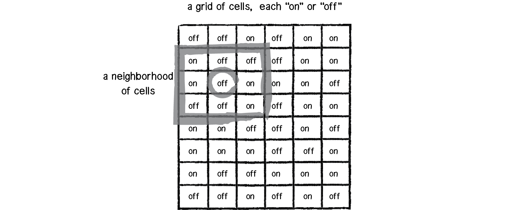
Figure 7.1

The development of cellular automata systems is typically attributed to Stanisław Ulam and John von Neumann, who were both researchers at the Los Alamos National Laboratory in New Mexico in the 1940s. Ulam was studying the growth of crystals and von Neumann was imagining a world of self-replicating robots. That’s right, robots that build copies of themselves. Once we see some examples of CA visualized, it’ll be clear how one might imagine modeling crystal growth; the robots idea is perhaps less obvious. Consider the design of a robot as a pattern on a grid of cells (think of filling in some squares on a piece of graph paper). Now consider a set of simple rules that would allow that pattern to create copies of itself on that grid. This is essentially the process of a CA that exhibits behavior similar to biological reproduction and evolution. (Incidentally, von Neumann’s cells had twenty-nine possible states.) Von Neumann’s work in self-replication and CA is conceptually similar to what is probably the most famous cellular automaton: the “Game of Life,” which we will discuss in detail in section 7.3.

Perhaps the most significant scientific (and lengthy) work studying cellular automata arrived in 2002: Stephen Wolfram’s 1,280-page A New Kind of Science. Available in its entirety for free online, Wolfram’s book discusses how CA are not simply neat tricks, but are relevant to the study of biology, chemistry, physics, and all branches of science. This chapter will barely scratch the surface of the theories Wolfram outlines (we will focus on the code implementation) so if the examples provided spark your curiosity, you’ll find plenty more to read about in his book.

7.2 Elementary Cellular Automata

The examples in this chapter will begin with a simulation of Wolfram’s work. To understand Wolfram’s elementary CA, we should ask ourselves the question: “What is the simplest cellular automaton we can imagine?” What’s exciting about this question and its answer is that even with the simplest CA imaginable, we will see the properties of complex systems at work.

Let’s build Wolfram’s elementary CA from scratch. Concepts first, then code. What are the three key elements of a CA?

1) Grid. The simplest grid would be one-dimensional: a line of cells.

Figure 7.2

2) States. The simplest set of states (beyond having only one state) would be two states: 0 or 1.

Figure 7.3

3) Neighborhood. The simplest neighborhood in one dimension for any given cell would be the cell itself and its two adjacent neighbors: one to the left and one to the right.

Figure 7.4: A neighborhood is three cells.

So we begin with a line of cells, each with an initial state (let’s say it is random), and each with two neighbors. We’ll have to figure out what we want to do with the cells on the edges (since those have only one neighbor each), but this is something we can sort out later.

Figure 7.5: The edge cell only has a neighborhood of two.

We haven’t yet discussed, however, what is perhaps the most important detail of how cellular automata work—time. We’re not really talking about real-world time here, but about the CA living over a period of time, which could also be called a generation and, in our case, will likely refer to the frame count of an animation. The figures above show us the CA at time equals 0 or generation 0. The questions we have to ask ourselves are: How do we compute the states for all cells at generation 1? And generation 2? And so on and so forth.

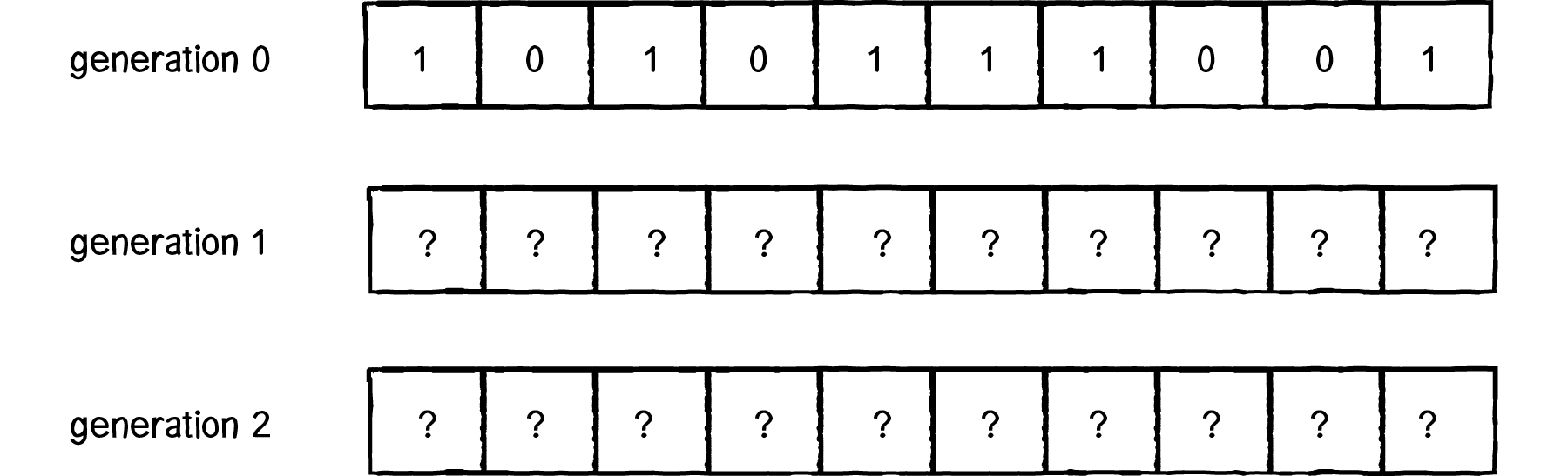
Figure 7.6

Let’s say we have an individual cell in the CA, and let’s call it CELL. The formula for calculating CELL’s state at any given time t is as follows:

CELL state at time t = f(CELL neighborhood at time t - 1)

In other words, a cell’s new state is a function of all the states in the cell’s neighborhood at the previous moment in time (or during the previous generation). We calculate a new state value by looking at all the previous neighbor states.

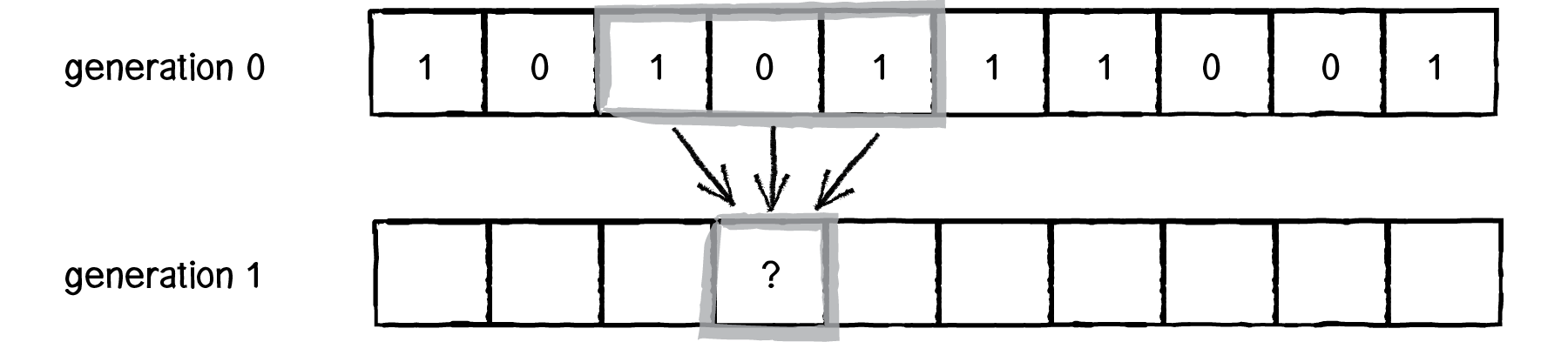
Figure 7.7

Now, in the world of cellular automata, there are many ways we could compute a cell’s state from a group of cells. Consider blurring an image. (Guess what? Image processing works with CA-like rules.) A pixel’s new state (i.e. its color) is the average of all of its neighbors’ colors. We could also say that a cell’s new state is the sum of all of its neighbors’ states. With Wolfram’s elementary CA, however, we can actually do something a bit simpler and seemingly absurd: We can look at all the possible configurations of a cell and its neighbor and define the state outcome for every possible configuration. It seems ridiculous—wouldn’t there be way too many possibilities for this to be practical? Let’s give it a try.

We have three cells, each with a state of 0 or 1. How many possible ways can we configure the states? If you love binary, you’ll notice that three cells define a 3-bit number, and how high can you count with 3 bits? Up to 8. Let’s have a look.

Figure 7.8

Once we have defined all the possible neighborhoods, we need to define an outcome (new state value: 0 or 1) for each neighborhood configuration.

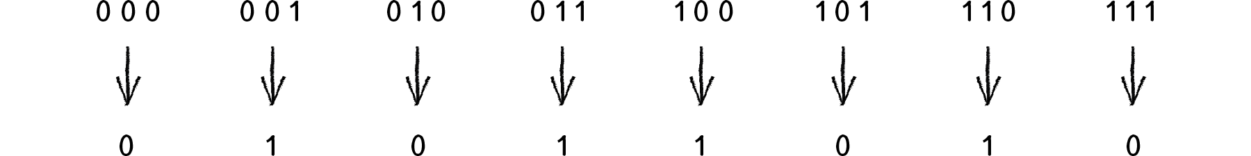
Figure 7.9

The standard Wolfram model is to start generation 0 with all cells having a state of 0 except for the middle cell, which should have a state of 1.

Figure 7.10

Referring to the ruleset above, let’s see how a given cell (we’ll pick the center one) would change from generation 0 to generation 1.

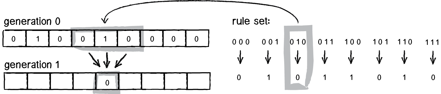
Figure 7.11

Try applying the same logic to all of the cells above and fill in the empty cells.

Now, let’s go past just one generation and color the cells —0 means white, 1 means black—and stack the generations, with each new generation appearing below the previous one.

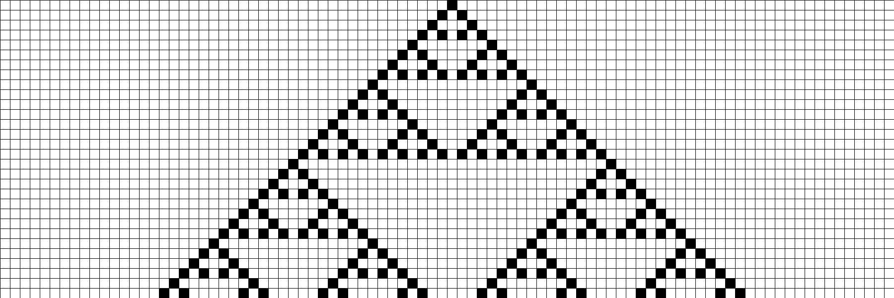
Figure 7.12: Rule 90

The low-resolution shape we’re seeing above is the “Sierpiński triangle.” Named after the Polish mathematician Wacław Sierpiński, it’s a fractal pattern that we’ll examine in the next chapter. That’s right: this incredibly simple system of 0s and 1s, with little neighborhoods of three cells, can generate a shape as sophisticated and detailed as the Sierpiński triangle. Let’s look at it again, only with each cell a single pixel wide so that the resolution is much higher.

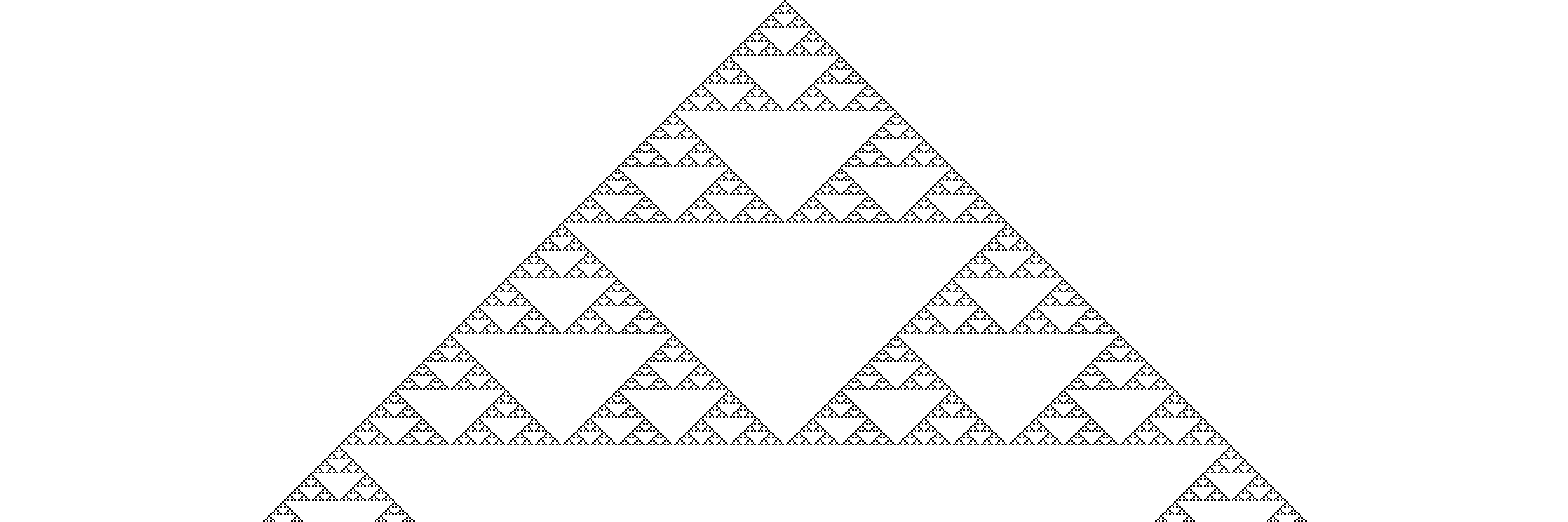
Figure 7.13: Rule 90

This particular result didn’t happen by accident. I picked this set of rules because of the pattern it generates. Take a look at Figure 7.8 one more time. Notice how there are eight possible neighborhood configurations; we therefore define a “ruleset” as a list of 8 bits.

So this particular rule can be illustrated as follows:

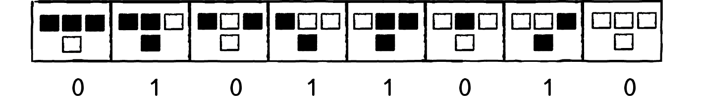
Figure 7.14: Rule 90

Eight 0s and 1s means an 8-bit number. How many combinations of eight 0s and 1s are there? 256. This is just like how we define the components of an RGB color. We get 8 bits for red, green, and blue, meaning we make colors with values from 0 to 255 (256 possibilities).

In terms of a Wolfram elementary CA, we have now discovered that there are 256 possible rulesets. The above ruleset is commonly referred to as “Rule 90” because if you convert the binary sequence—01011010—to a decimal number, you’ll get the integer 90. Let’s try looking at the results of another ruleset.

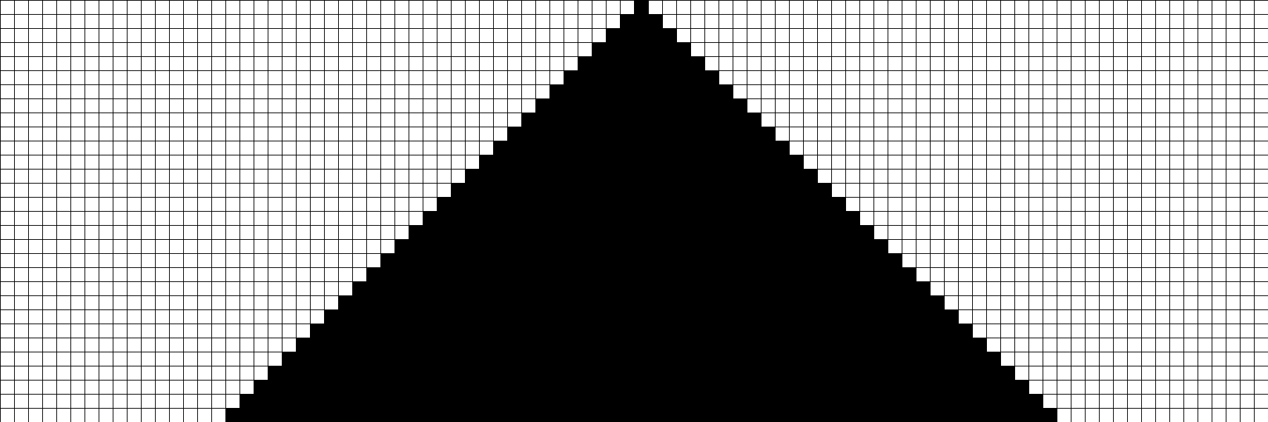
Figure 7.15: Rule 222

Figure 7.16: A Textile Cone Snail (Conus textile), Cod Hole, Great Barrier Reef, Australia, 7 August 2005. Photographer: Richard Ling richard@research.canon.com.au

As we can now see, the simple act of creating a CA and defining a ruleset does not guarantee visually interesting results. Out of all 256 rulesets, only a handful produce compelling outcomes. However, it’s quite incredible that even one of these rulesets for a one-dimensional CA with only two possible states can produce the patterns we see every day in nature (see Figure 7.16), and it demonstrates how valuable these systems can be in simulation and pattern generation.

Before we go too far down the road of how Wolfram classifies the results of varying rulesets, let’s look at how we actually build a Processing sketch that generates the Wolfram CA and visualizes it onscreen.

7.3 How to Program an Elementary CA

You may be thinking: “OK, I’ve got this cell thing. And the cell thing has some properties, like a state, what generation it’s on, who its neighbors are, where it lives pixel-wise on the screen. And maybe it has some functions: it can display itself, it can generate its new state, etc.” This line of thinking is an excellent one and would likely lead you to write some code like this:

class Cell {
 
}

This line of thinking, however, is not the road we will first travel. Later in this chapter, we will discuss why an object-oriented approach could prove valuable in developing a CA simulation, but to begin, we can work with a more elementary data structure. After all, what is an elementary CA but a list of 0s and 1s? Certainly, we could describe the following CA generation using an array:

Figure 7.17

int[] cells = {1,0,1,0,0,0,0,1,0,1,1,1,0,0,0,1,1,1,0,0};

To draw that array, we simply check if we’ve got a 0 or a 1 and create a fill accordingly.

for (int i = 0; i < cells.length; i++) {
  if (cells[i] == 0) fill(255);

  else fill(0);
  stroke(0);
  rect(i*50,0,50,50);
}

Now that we have the array to describe the cell states of a given generation (which we’ll ultimately consider the “current” generation), we need a mechanism by which to compute the next generation. Let’s think about the pseudocode of what we are doing at the moment.

For every cell in the array:

This may lead you to write some code like this:

for (int i = 0; i < cells.length; i++) {
 

  int left   = cell[i-1];
  int middle = cell[i];
  int right  = cell[i+1];

  int newstate = rules(left,middle,right);
 

  cell[i] = newstate;
}

We’re fairly close to getting this right, but we’ve made one minor blunder and one major blunder in the above code. Let’s talk about what we’ve done well so far.

Notice how easy it is to look at a cell’s neighbors. Because an array is an ordered list of data, we can use the fact that the indices are numbered to know which cells are next to which cells. We know that cell number 15, for example, has cell 14 to its left and 16 to its right. More generally, we can say that for any cell i, its neighbors are i-1 and i+1.

We’re also farming out the calculation of a new state value to some function called rules(). Obviously, we’re going to have to write this function ourselves, but the point we’re making here is modularity. We have a basic framework for the CA in this function, and if we later want to change how the rules operate, we don’t have to touch that framework; we can simply rewrite the rules() function to compute the new states differently.

So what have we done wrong? Let’s talk through how the code will execute. First, we look at cell index i equals 0. Now let’s look at 0’s neighbors. Left is index -1. Middle is index 0. And right is index 1. However, our array by definition does not have an element with the index -1. It starts with 0. This is a problem we’ve alluded to before: the edge cases.

How do we deal with the cells on the edge who don’t have a neighbor to both their left and their right? Here are three possible solutions to this problem:

To make the code easiest to read and understand right now, we’ll go with option #1 and just skip the edge cases, leaving their values constant. This can be accomplished by starting the loop one cell later and ending one cell earlier:

for (int i = 1; i < cells.length-1; i++) {
  int left   = cell[i-1];
  int middle = cell[i];
  int right  = cell[i+1];
  int newstate = rules(left,middle,right);
  cell[i] = newstate;
}

There’s one more problem we have to fix before we’re done. It’s subtle and you won’t get a compilation error; the CA just won’t perform correctly. However, identifying this problem is absolutely fundamental to the techniques behind programming CA simulations. It all lies in this line of code:

  cell[i] = newstate;

This seems like a perfectly innocent line. After all, we’ve computed the new state value and we’re simply giving the cell its new state. But in the next iteration, you’ll discover a massive bug. Let’s say we’ve just computed the new state for cell #5. What do we do next? We calculate the new state value for cell #6.

Cell #6, generation 0 = some state, 0 or 1
Cell #6, generation 1 = a function of states for cell #5, cell #6, and cell #7 at *generation 0*

Notice how we need the value of cell #5 at generation 0 in order to calculate cell #6’s new state at generation 1? A cell’s new state is a function of the previous neighbor states. Do we know cell #5’s value at generation 0? Remember, Processing just executes this line of code for i = 5.

  cell[i] = newstate;

Once this happens, we no longer have access to cell #5’s state at generation 0, and cell index 5 is storing the value for generation 1. We cannot overwrite the values in the array while we are processing the array, because we need those values to calculate the new values. A solution to this problem is to have two arrays, one to store the current generation states and one for the next generation states.

int[] newcells = new int[cells.length];
 
for (int i = 1; i < cells.length-1; i++) {

  int left   = cell[i-1];
  int middle = cell[i];
  int right  = cell[i+1];

  int newstate = rules(left,middle,right);

  newcells[i] = newstate;
}

Once the entire array of values is processed, we can then discard the old array and set it equal to the new array of states.

cells = newcells;

We’re almost done. The above code is complete except for the fact that we haven’t yet written the rules() function that computes the new state value based on the neighborhood (left, middle, and right cells). We know that function needs to return an integer (0 or 1) as well as receive three arguments (for the three neighbors).

  int rules (int a, int b, int c) {

Now, there are many ways we could write this function, but I’d like to start with a long-winded one that will hopefully provide a clear illustration of what we are doing.

Let’s first establish how we are storing the ruleset. The ruleset, if you remember from the previous section, is a series of 8 bits (0 or 1) that defines that outcome for every possible neighborhood configuration.

Figure 7.14 (repeated)

We can store this ruleset in Processing as an array.

int[] ruleset = {0,1,0,1,1,0,1,0};

And then say:

if (a == 1 && b == 1 && c == 1) return ruleset[0];

If left, middle, and right all have the state 1, then that matches the configuration 111 and the new state should be equal to the first value in the ruleset array. We can now duplicate this strategy for all eight possibilities.

  int rules (int a, int b, int c) {
    if      (a == 1 && b == 1 && c == 1) return ruleset[0];
    else if (a == 1 && b == 1 && c == 0) return ruleset[1];
    else if (a == 1 && b == 0 && c == 1) return ruleset[2];
    else if (a == 1 && b == 0 && c == 0) return ruleset[3];
    else if (a == 0 && b == 1 && c == 1) return ruleset[4];
    else if (a == 0 && b == 1 && c == 0) return ruleset[5];
    else if (a == 0 && b == 0 && c == 1) return ruleset[6];
    else if (a == 0 && b == 0 && c == 0) return ruleset[7];

    return 0;
  }

I like having the example written as above because it describes line by line exactly what is happening for each neighborhood configuration. However, it’s not a great solution. After all, what if we design a CA that has 4 possible states (0-3) and suddenly we have 64 possible neighborhood configurations? With 10 possible states, we have 1,000 configurations. Certainly we don’t want to type in 1,000 lines of code!

Another solution, though perhaps a bit more difficult to follow, is to convert the neighborhood configuration (a 3-bit number) into a regular integer and use that value as the index into the ruleset array. This can be done in Java like so.

  int rules (int a, int b, int c) {

    String s = "" + a + b + c;
 

    int index = Integer.parseInt(s,2);
 
    return ruleset[index];
  }

There’s one tiny problem with this solution, however. Let’s say we are implementing rule 222:

int[] ruleset = {1,1,0,1,1,1,1,0};

And we have the neighborhood “111”. The resulting state is equal to ruleset index 0, as we see in the first way we wrote the function.

    if (a == 1 && b == 1 && c == 1) return ruleset[0];

If we convert “111” to a decimal number, we get 7. But we don’t want ruleset[7]; we want ruleset[0]. For this to work, we need to write the ruleset with the bits in reverse order, i.e.

int[] ruleset = {0,1,1,1,1,0,1,1};

So far in this section, we’ve written everything we need to compute the generations for a Wolfram elementary CA. Let’s take a moment to organize the above code into a class, which will ultimately help in the design of our overall sketch.

class CA {

  int[] cells;
  int[] ruleset;

 
  CA() {
    cells = new int[width];

    ruleset = {0,1,0,1,1,0,1,0};
 
    for (int i = 0; i < cells.length; i++) {
      cells[i] = 0;
    }

    cells[cells.length/2] = 1;
  }
 
  void generate() {

    int[] nextgen = new int[cells.length];
    for (int i = 1; i < cells.length-1; i++) {
      int left   = cells[i-1];
      int me     = cells[i];
      int right  = cells[i+1];
      nextgen[i] = rules(left, me, right);
    }

    cells = nextgen;
  }
 

  int rules (int a, int b, int c) {
    String s = "" + a + b + c;
    int index = Integer.parseInt(s,2);
    return ruleset[index];
  }

}

7.4 Drawing an Elementary CA

What’s missing? Presumably, it’s our intention to display cells and their states in visual form. As we saw earlier, the standard technique for doing this is to stack the generations one on top of each other and draw a rectangle that is black (for state 1) or white (for state 0).

Figure 7.12 (repeated)

Before we implement this particular visualization, I’d like to point out two things.

One, this visual interpretation of the data is completely literal. It’s useful for demonstrating the algorithms and results of Wolfram’s elementary CA, but it shouldn’t necessarily drive your own personal work. It’s rather unlikely that you are building a project that needs precisely this algorithm with this visual style. So while learning to draw the CA in this way will help you understand and implement CA systems, this skill should exist only as a foundation.

Second, the fact that we are visualizing a one-dimensional CA with a two-dimensional image can be confusing. It’s very important to remember that this is not a 2D CA. We are simply choosing to show a history of all the generations stacked vertically. This technique creates a two-dimensional image out of many instances of one-dimensional data. But the system itself is one-dimensional. Later, we are going to look at an actual 2D CA (the Game of Life) and discuss how we might choose to display such a system.

The good news is that drawing the CA is not particularly difficult. Let’s begin by looking at how we would render a single generation. Assume we have a Processing window 600 pixels wide and we want each cell to be a 10x10 square. We therefore have a CA with 60 cells. Of course, we can calculate this value dynamically.

int w = 10;

int[] cells = new int[width/w];

Assuming we’ve gone through the process of generating the cell states (which we did in the previous section), we can now loop through the entire array of cells, drawing a black cell when the state is 1 and a white one when the state is 0.

for (int i = 0; i < cells.length; i++) {

  if (cells[i] == 1) fill(0);
  else               fill(255);

  rect(i*w, 0, w, w);
}

In truth, we could optimize the above by having a white background and only drawing when there is a black cell (saving us the work of drawing many white squares), but in most cases this solution is good enough (and necessary for other more sophisticated designs with varying colors, etc.) Also, if we wanted each cell to be represented as a single pixel, we would not want to use Processing’s rect() function, but rather access the pixel array directly.

In the above code, you’ll notice the y-location for each rectangle is 0. If we want the generations to be drawn next to each other, with each row of cells marking a new generation, we’ll also need to compute a y-location based on how many iterations of the CA we’ve executed. We could accomplish this by adding a “generation” variable (an integer) to our CA class and incrementing it each time through generate(). With these additions, we can now look at the CA class with all the features for both computing and drawing the CA.

Example 7.1: Wolfram elementary cellular automata

class CA {
  int[] cells;
  int[] ruleset;
  int w = 10;

  int generation = 0;
  CA() {
    cells = new int[width/w];
    ruleset = {0,1,0,1,1,0,1,0};
    cells[cells.length/2] = 1;
  }
 

  void generate() {
    int[] nextgen = new int[cells.length];
    for (int i = 1; i < cells.length-1; i++) {
      int left   = cells[i-1];
      int me     = cells[i];
      int right  = cells[i+1];
      nextgen[i] = rules(left, me, right);
    }
    cells = nextgen;

    generation++;
  }
 
  int rules(int a, int b, int c) {
    String s = "" + a + b + c;
    int index = Integer.parseInt(s,2);
    return ruleset[index];
  }
 
  for (int i = 0; i < cells.length; i++) {
    if (cells[i] == 1) fill(0);
    else               fill(255);

    rect(i*w, generation*w, w, w);
  }
}

7.5 Wolfram Classification

Before we move on to looking at CA in two dimensions, it’s worth taking a brief look at Wolfram’s classification for cellular automata. As we noted earlier, the vast majority of elementary CA rulesets produce uninspiring results, while some result in wondrously complex patterns like those found in nature. Wolfram has divided up the range of outcomes into four classes:

Class 1: Uniformity. Class 1 CAs end up, after some number of generations, with every cell constant. This is not terribly exciting to watch. Rule 222 (above) is a class 1 CA; if you run it for enough generations, every cell will eventually become and remain black.

Class 2: Repetition. Like class 1 CAs, class 2 CAs remain stable, but the cell states are not constant. Rather, they oscillate in some regular pattern back and forth from 0 to 1 to 0 to 1 and so on. In rule 190 (above), each cell follows the sequence 11101110111011101110.

Class 3: Random. Class 3 CAs appear random and have no easily discernible pattern. In fact, rule 30 (above) is used as a random number generator in Wolfram’s Mathematica software. Again, this is a moment where we can feel amazed that such a simple system with simple rules can descend into a chaotic and random pattern.

Class 4: Complexity. Class 4 CAs can be thought of as a mix between class 2 and class 3. One can find repetitive, oscillating patterns inside the CA, but where and when these patterns appear is unpredictable and seemingly random. Class 4 CAs exhibit the properties of complex systems that we described earlier in this chapter and in Chapter 6. If a class 3 CA wowed you, then a class 4 like Rule 110 above should really blow your mind.

7.6 The Game of Life

The next step we are going to take is to move from a one-dimensional CA to a two-dimensional one. This will introduce some additional complexity; each cell will have a bigger neighborhood, but that will open up the door to a range of possible applications. After all, most of what we do in computer graphics lives in two dimensions, and this chapter will demonstrate how to apply CA thinking to what we draw in our Processing sketches.

In 1970, Martin Gardner wrote an article in Scientific American that documented mathematician John Conway’s new “Game of Life,” describing it as “recreational” mathematics and suggesting that the reader get out a chessboard and some checkers and “play.” While the Game of Life has become something of a computational cliché (make note of the myriad projects that display the Game of Life on LEDs, screens, projection surfaces, etc.), it is still important for us to build it from scratch. For one, it provides a good opportunity to practice our skills with two-dimensional arrays, object orientation, etc. But perhaps more importantly, its core principles are tied directly to our core goals—simulating the natural world with code. Though we may want to avoid simply duplicating it without a great deal of thought or care, the algorithm and its technical implementation will provide us with the inspiration and foundation to build simulations that exhibit the characteristics and behaviors of biological systems of reproduction.

Unlike von Neumann, who created an extraordinarily complex system of states and rules, Conway wanted to achieve a similar “lifelike” result with the simplest set of rules possible. Martin Gardner outlined Conway’s goals as follows:

“1. There should be no initial pattern for which there is a simple proof that the population can grow without limit. 2. There should be initial patterns that apparently do grow without limit. 3. There should be simple initial patterns that grow and change for a considerable period of time before coming to an end in three possible ways: fading away completely (from overcrowding or becoming too sparse), settling into a stable configuration that remains unchanged thereafter, or entering an oscillating phase in which they repeat an endless cycle of two or more periods.” —Martin Gardner, Scientific American 223 (October 1970): 120-123.

The above might sound a bit cryptic, but it essentially describes a Wolfram class 4 CA. The CA should be patterned but unpredictable over time, eventually settling into a uniform or oscillating state. In other words, though Conway didn’t use this terminology, it should have all those properties of a complex system that we keep mentioning.

Let’s look at how the Game of Life works. It won’t take up too much time or space, since we’ve covered the basics of CA already.

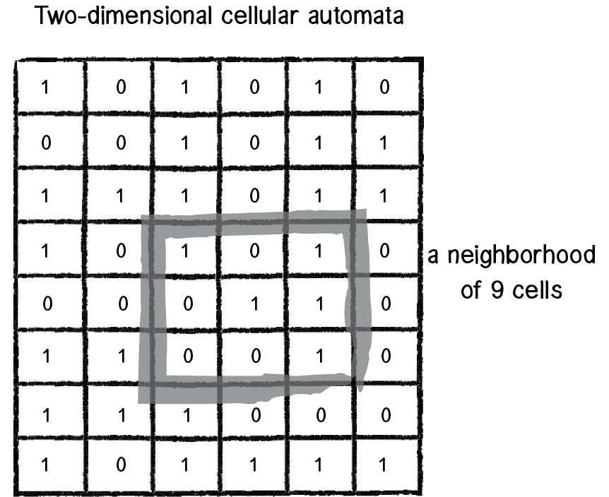
Figure 7.22

First, instead of a line of cells, we now have a two-dimensional matrix of cells. As with the elementary CA, the possible states are 0 or 1. Only in this case, since we’re talking about “life," 0 means dead and 1 means alive.

The cell’s neighborhood has also expanded. If a neighbor is an adjacent cell, a neighborhood is now nine cells instead of three.

With three cells, we had a 3-bit number or eight possible configurations. With nine cells, we have 9 bits, or 512 possible neighborhoods. In most cases, it would be impractical to define an outcome for every single possibility. The Game of Life gets around this problem by defining a set of rules according to general characteristics of the neighborhood. In other words, is the neighborhood overpopulated with life? Surrounded by death? Or just right? Here are the rules of life.

Let’s look at a few examples.

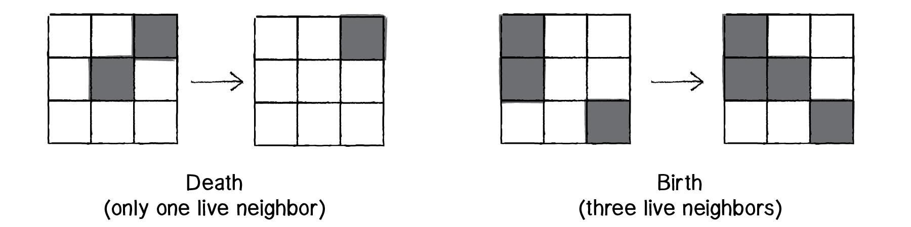
Figure 7.23

With the elementary CA, we were able to look at all the generations next to each other, stacked as rows in a 2D grid. With the Game of Life, however, the CA itself is in two dimensions. We could try creating an elaborate 3D visualization of the results and stack all the generations in a cube structure (and in fact, you might want to try this as an exercise). Nevertheless, the typical way the Game of Life is displayed is to treat each generation as a single frame in an animation. So instead of viewing all the generations at once, we see them one at a time, and the result resembles rapidly growing bacteria in a petri dish.

One of the exciting aspects of the Game of Life is that there are initial patterns that yield intriguing results. For example, some remain static and never change.

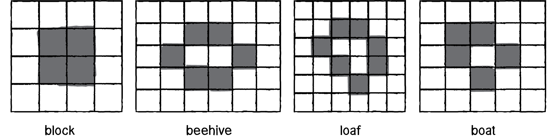
Figure 7.24

There are patterns that oscillate back and forth between two states.

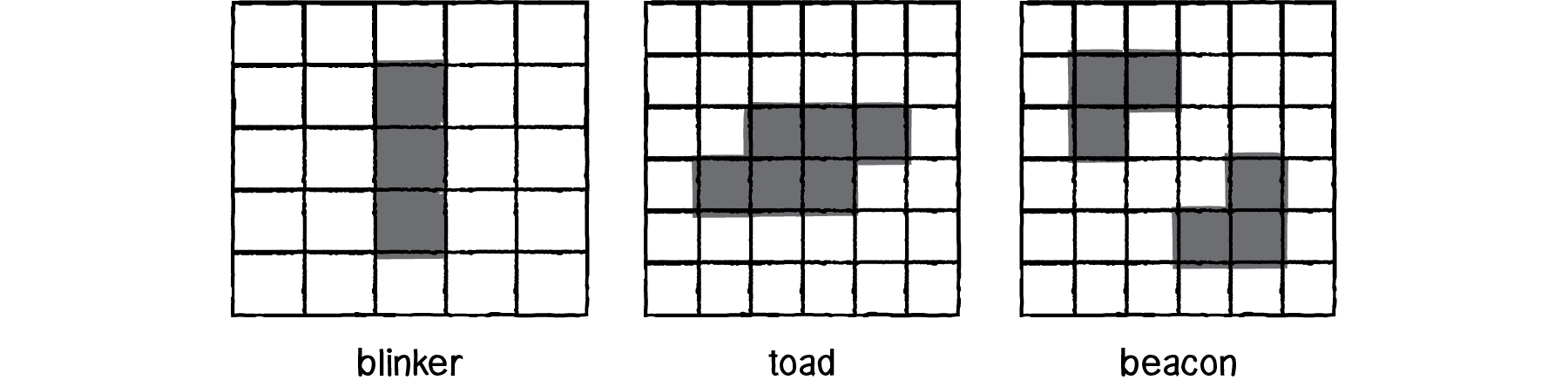
Figure 7.25

And there are also patterns that from generation to generation move about the grid. (It’s important to note that the cells themselves aren’t actually moving, although we see the appearance of motion in the result as the cells turn on and off.)

Figure 7.26

If you are interested in these patterns, there are several good “out of the box” Game of Life demonstrations online that allow you to configure the CA’s initial state and watch it run at varying speeds. Two examples you might want to examine are:

For the example we’ll build from scratch in the next section, it will be easier to simply randomly set the states for each cell.

7.7 Programming the Game of Life

Now we just need to extend our code from the Wolfram CA to two dimensions. We used a one-dimensional array to store the list of cell states before, and for the Game of Life, we can use a two-dimensional array.

int[][] board = new int[columns][rows];

We’ll begin by initializing each cell of the board with a random state: 0 or 1.

for (int x = 0; x < columns; x++) {
  for (int y = 0; y < rows; y++) {

    current[x][y] = int(random(2));
  }
}

And to compute the next generation, just as before, we need a fresh 2D array to write to as we analyze each cell’s neighborhood and calculate a new state.

int[][] next = new int[columns][rows];
 
for (int x = 0; x < columns; x++) {
  for (int y = 0; y < rows; y++) {
 

    next[x][y] = _______________?;
 
  }
}

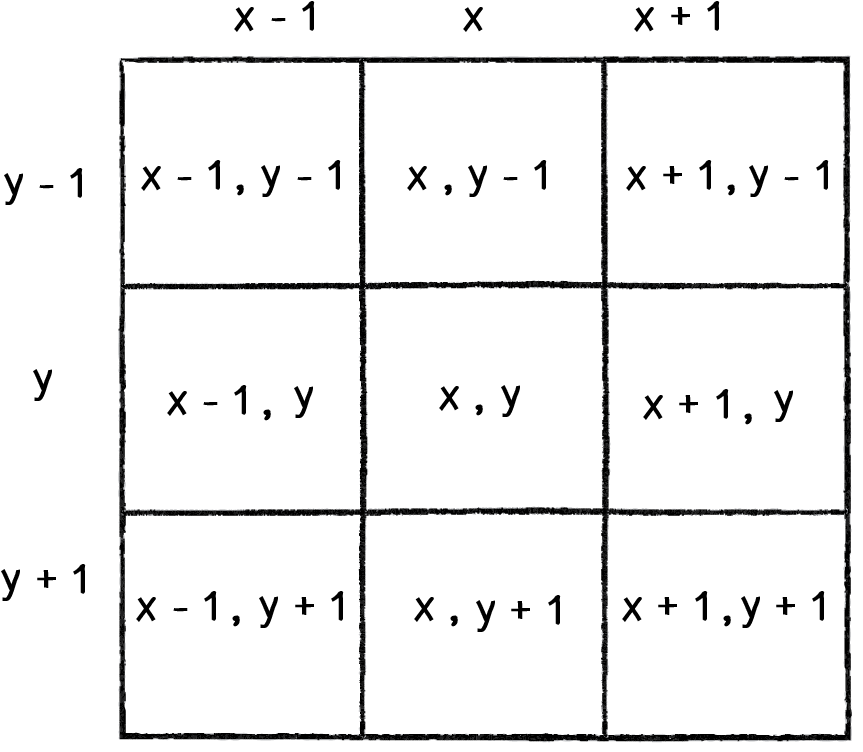
Figure 7.27

OK. Before we can sort out how to actually calculate the new state, we need to know how we can reference each cell’s neighbor. In the case of the 1D CA, this was simple: if a cell index was i, its neighbors were i-1 and i+1. Here each cell doesn’t have a single index, but rather a column and row index: x,y. As shown in Figure 7.27, we can see that its neighbors are: (x-1,y-1) (x,y-1), (x+1,y-2), (x-1,y), (x+1,y), (x-1,y+1), (x,y+1), and (x+1,y+1).

All of the Game of Life rules operate by knowing how many neighbors are alive. So if we create a neighbor counter variable and increment it each time we find a neighbor with a state of 1, we’ll have the total of live neighbors.

int neighbors = 0;
 

if (board[x-1][y-1] == 1) neighbors++;
if (board[x  ][y-1] == 1) neighbors++;
if (board[x+1][y-1] == 1) neighbors++;

if (board[x-1][y]   == 1) neighbors++;
if (board[x+1][y]   == 1) neighbors++;

if (board[x-1][y+1] == 1) neighbors++;
if (board[x  ][y+1] == 1) neighbors++;
if (board[x+1][y+1] == 1) neighbors++;

And again, just as with the Wolfram CA, we find ourselves in a situation where the above is a useful and clear way to write the code for teaching purposes, allowing us to see every step (each time we find a neighbor with a state of one, we increase a counter). Nevertheless, it’s a bit silly to say, “If the cell state equals one, add one to a counter” when we could just say, “Add the cell state to a counter.” After all, if the state is only a 0 or 1, the sum of all the neighbors’ states will yield the total number of live cells. Since the neighbors are arranged in a mini 3x3 grid, we can add them all up with another loop.

for (int i = -1; i <= 1; i++) {
  for (int j = -1; j <= 1; j++) {

    neighbors += board[x+i][y+j];
   }
}

Of course, we’ve made a mistake in the code above. In the Game of Life, the cell itself does not count as one of the neighbors. We could use a conditional to skip adding the state when both i and j equal 0, but another option would be to just subtract the cell state once we’ve finished the loop.

neighbors -= board[x][y];

Finally, once we know the total number of live neighbors, we can decide what the cell’s new state should be according to the rules: birth, death, or stasis.

if      ((board[x][y] == 1) && (neighbors <  2)) {
  next[x][y] = 0;
}

else if ((board[x][y] == 1) && (neighbors >  3)) {
  next[x][y] = 0;
}

else if ((board[x][y] == 0) && (neighbors == 3)) {
  next[x][y] = 1;
}

else {
  next[x][y] = board[x][y];
}

Putting this all together, we have:

int[][] next = new int[columns][rows];
 

for (int x = 1; x < columns-1; x++) {
  for (int y = 1; y < rows-1; y++) {

    int neighbors = 0;
    for (int i = -1; i <= 1; i++) {
      for (int j = -1; j <= 1; j++) {
        neighbors += board[x+i][y+j];
      }
    }
 

    neighbors -= board[x][y];
 

 
    if      ((board[x][y] == 1) && (neighbors <  2)) next[x][y] = 0;
    else if ((board[x][y] == 1) && (neighbors >  3)) next[x][y] = 0;
    else if ((board[x][y] == 0) && (neighbors == 3)) next[x][y] = 1;
    else next[x][y] = board[x][y];

  }
}
 

board = next;

Finally, once the next generation is calculated, we can employ the same method we used to draw the Wolfram CA—a square for each spot, white for off, black for on.

Example 7.2: Game of Life

for ( int i = 0; i < columns;i++) {
  for ( int j = 0; j < rows;j++) {
 

    if ((board[i][j] == 1)) fill(0);

    else fill(255);
    stroke(0);
 
    rect(i*w, j*w, w, w);
  }
}

7.8 Object-Oriented Cells

Over the course of the previous six chapters, we’ve slowly built examples of systems of objects with properties that move about the screen. And in this chapter, although we’ve been talking about a “cell” as if it were an object, we actually haven’t been using any object orientation in our code (other than a class to describe the CA system as a whole). This has worked because a cell is such an enormously simple object (a single bit). However, in a moment, we are going to discuss some ideas for further developing CA systems, many of which involve keeping track of multiple properties for each cell. For example, what if a cell needed to remember its last ten states? Or what if we wanted to apply some of our motion and physics thinking to a CA and have the cells move about the window, dynamically changing their neighbors from frame to frame?

To accomplish any of these ideas (and more), it would be helpful to see how we might treat a cell as an object with multiple properties, rather than as a single 0 or 1. To show this, let’s just recreate the Game of Life simulation. Only instead of:

  int[][] board;

Let’s have:

  Cell[][] board;

where Cell is a class we will write. What are the properties of a Cell object? In our Game of Life example, each cell has a location and size, as well as a state.

class Cell {
 

  float x, y;
  float w;

  int state;

In the non-OOP version, we used a separate 2D array to keep track of the states for the current and next generation. By making a cell an object, however, each cell could keep track of both states. In this case, we’ll think of the cell as remembering its previous state (for when new states need to be computed).

  int previous;

This allows us to visualize more information about what the state is doing. For example, we could choose to color a cell differently if its state has changed. For example:

Example 7.3: Game of Life OOP

void display() {

  if (previous == 0 && state == 1) fill(0,0,255);
  else if (state == 1) fill(0);
 

  else if (previous == 1 && state == 0) fill(255,0,0);
  else fill(255);
 
  rect(x, y, w, w);
}

Not much else about the code (at least for our purposes here) has to change. The neighbors can still be counted the same way; the difference is that we now need to refer to the object’s state variables as we loop through the 2D array.

for (int x = 1; x < columns-1; x++) {
  for (int y = 1; y < rows-1; y++) {
 
    int neighbors = 0;
    for (int i = -1; i <= 1; i++) {
      for (int j = -1; j <= 1; j++) {

        neighbors += board[x+i][y+j].previous;
      }
    }
    neighbors -= board[x][y].previous;
 

 
 
    if      ((board[x][y].state == 1) && (neighbors <  2)) board[x][y].newState(0);
    else if ((board[x][y].state == 1) && (neighbors >  3)) board[x][y].newState(0);
    else if ((board[x][y].state == 0) && (neighbors == 3)) board[x][y].newState(1);

  }
}

7.9 Variations of Traditional CA

Now that we have covered the basic concepts, algorithms, and programming strategies behind the most famous 1D and 2D cellular automata, it’s time to think about how you might take this foundation of code and build on it, developing creative applications of CAs in your own work. In this section, we’ll talk through some ideas for expanding the features of the CA examples. Example answers to each of these exercises can be found on the book website.

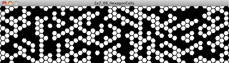
1) Non-rectangular Grids. There’s no particular reason why you should limit yourself to having your cells on a rectangular grid. What happens if you design a CA with another type of shape?

Exercise 7.9

Create a CA using a grid of hexagons (as below), each with six neighbors.

2) Probabilistic. The rules of a CA don’t necessarily have to define an exact outcome.

3) Continuous. We’ve looked at examples where the cell’s state can only be a 1 or a 0. But what if the cell’s state was a floating point number between 0 and 1?

4) Image Processing. We briefly touched on this earlier, but many image-processing algorithms operate on CA-like rules. Blurring an image is creating a new pixel out of the average of a neighborhood of pixels. Simulations of ink dispersing on paper or water rippling over an image can be achieved with CA rules.

5) Historical. In the Game of Life object-oriented example, we used two variables to keep track of its state: current and previous. What if you use an array to keep track of a cell’s state history? This relates to the idea of a “complex adaptive system,” one that has the ability to adapt and change its rules over time by learning from its history. We’ll see an example of this in Chapter 10: Neural Networks.

6) Moving cells. In these basic examples, cells have a fixed position on a grid, but you could build a CA with cells that have no fixed position and instead move about the screen.

7) Nesting. Another feature of complex systems is that they can be nested. Our world tends to work this way: a city is a complex system of people, a person is a complex system of organs, an organ is a complex system of cells, and so on and so forth.